Comparing GC Collectors
Automatic memory management through advanced Garbage Collection has been one of the main selling points for Java and the JVM from the beginning. We can simply create the objects we need and the JVM makes sure they are removed when no longer in use. The garbage collector can be tuned and configured in a wide variety of ways. But how do you know what options work best for your application?
In this article I look at the alternative garbage collectors that are available in the JVM and try to identify the differences between them. I show how you can compare them for your application and choose the one that makes most sense for your needs.
GC Tuning Overview
When tuning garbage collection performance it is interesting to look at what collectors are available in the platform, and what kind of goals we can achieve.
GC Goals
There are basically two primary measures of GC performance:
- Throughput - This is the percentage of total time not spent in garbage collection considered over long periods of time. So if the application spends 10% of its time in garbage collection the throughput is 90%. If you want your application to perform as many calculations as possible you typically want to tune the garbage collection to maximize throughput.
- Pause-times/latency - This is how long the application pauses/appears unresponsive because of garbage collection. It is interesting to consider both maximum pause time, and various statistics like average and standard deviation. If you want your application to be as responsive as possible you want to minimize the latency cause by garbage collection.
Another important factor is the footprint of the JVM. That is how much memory is commited by the JVM when running. The choice of collector, and tuning of the two goals metioned above, can influence what the optimal footprint of the application is.
Available Collectors
There are 4 available collectors in the Java HotSpot VM:
- The Serial collector uses a single thread to perform all garbage collection work. As such it works best on single processor machines, or on applications with small data sets (less than 100 MB).
- The Parallel collector performs minor collections in parallel. It is supposed to maximize the throughput of the application.
- The mostly concurrent collectors perform most of their work concurrently (without pausing the application). This is supposed to keep pauses short and minimize the latency. The Java HotSpot VM offers two mostly concurrent collectors:
- The Concurrent Mark Sweep (CMS) collector.
- The Garbage First (G1) collector.
In the following I will show a comparison of both throughput and latency for all 4 collectors in a simple test application.
Process and Tools
I have created a simple test-application that produces a lot of garbage. It runs for one minute before shutting itself down. The application was created using Dropwizard and can be seen on my github page.
I ran the test on my MacBook Pro with a 2.8GHz quad-core Intel Core i7 processor. The application is run with a maxium heap of 2G with full GC logging turned on. For example with the serial collector the application was started with these parameters:
java -Xmx2g -Xloggc:gc_serial.log -XX:+UseSerialGC -XX:+PrintGCDetails -XX:+PrintGCDateStamps eivindw.TestApp server
The only difference between the 4 runs is the name of the GC log file (-Xloggc:gc_<collector-name>.log) and the parameter to select the collector (-XX:+UseSerialGC, -XX:+UseParallelGC, -XX:+UseConcMarkSweepGC or -XX:+UseG1GC).
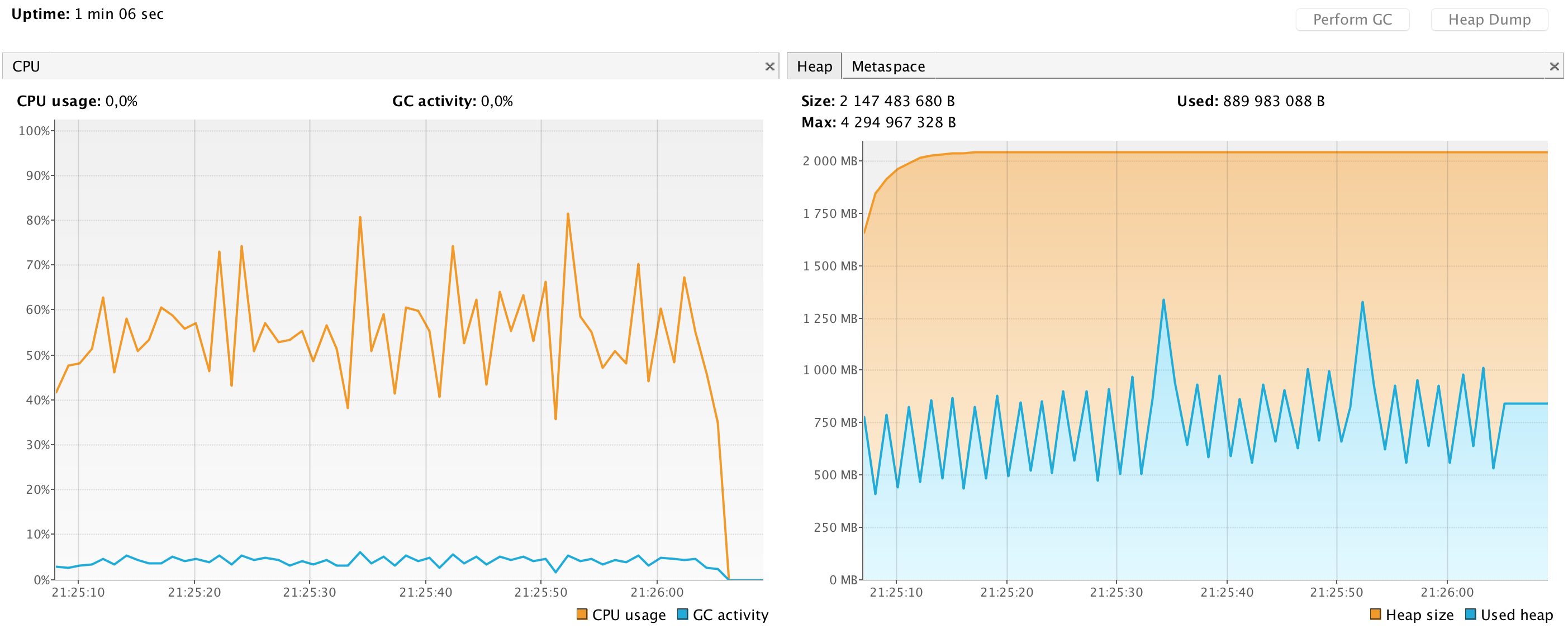
While the application is running I used Java VisualVM to create a graph showing CPU and memory usage. This gives us a nice visual way to compare the application running with the different collectors.
After running I used a tool called GCViewer to calculate statistics from the GC log. This creates a report with throughput, pause-times and other metrics. With logs and metrics from all 4 collectors we can compare numbers.
Results
The serial collector has low CPU consumption. It runs often and seems to do a good job at keeping the memory footprint low. It has only committed 50% of the 2GB available heap:

The parallel collector has a much higher CPU consumption than the serial collector, which is expected. It has a significant pattern in the memory usage graph, clearly showing the minor and major collection cycles.

The CMS collector has a much less regular pattern both in CPU usage and memory. It seems to be collecting much more memory in the minor collections than the parallel collector, but also has a few very big major collections.

The G1 collector has a significantly higher CPU consumption than all the other collectors. It has a very regular memory footprint, allocating max memory right after startup and keeping it at max. We can also clearly see that it runs small collection cycles constantly.
Comparison by numbers
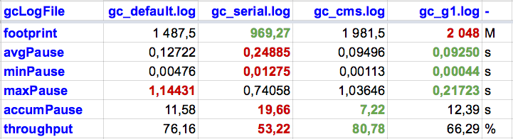
These are the numbers calculated from the GC logs, using the GCViewer tool.
Seems like the collectors deliver pretty close to what they promise for my little example application. The serial collector has the smallest memory footprint, but also the lowest throughput and worst (longest) average and minimum pause times. The parallel collector (gc_default.log in the table) has the second best throughput, but the worst maximum pause time. The CMS collector delivers, somewhat surprisingly, the best throughput in the test. CMS also has generally low pause times, except a few maximum pause times lasting more than a second. At last, the G1 collector has the best pause times (minimum, maximum and average), but delivers the second worst throughput in the test.
Conclusion
These tests shows a clear difference between the alternative collectors that can be chosen on the Java HotSpot VM. It is interesting to see how they utilize CPU and memory resources to achieve their goals.
The results shown here are of course only valid for my small example application. But the process and tools used are pretty much all you need to tune or monitor the GC performance of any JVM application. Just turn on detailed GC logging and run GCViewer or similar to calculate metrics. Choosing the best configuration for your application is then simply a matter of comparing metrics.